Lorenz attractor

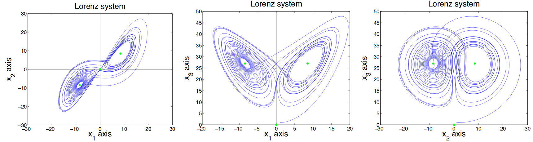
Consider the following Lorenz system of ODEs \begin{equation}\label{eq:lorenz} \boldsymbol y'(x) = \begin{bmatrix} y_1'\newline y_2'\newline y_3 \end{bmatrix} = \begin{bmatrix} -\alpha y_1+\alpha y_2, \newline -y_1y_3+\beta y_1- y_2, \newline y_1y_2-\gamma y_3. \end{bmatrix} = \begin{bmatrix} f_1(x,y_1,y_2,y_3)\newline f_2(x,y_1,y_2,y_3)\newline f_3(x,y_1,y_2,y_3) \end{bmatrix} = \boldsymbol f(x,\boldsymbol y) \end{equation}

Create a matlab function
```
function f = LORENZ(x,y,var)
```
(on a separate file) that implements the ODE (\ref{eq:lorenz}), with var containing the parameters $(\alpha, \beta, \gamma)$.
Implement the implicit Adams method with 6 steps as a solver for the system (\ref{eq:lorenz}). Use a predictor-corrector strategy, within a specific matlab function
```
function [x,y] = IAM6(FUNC,x0,xN,y0,N,var)
```
where y0 is a vector that contains sufficiently many starting values. Use the following explicit Adams method for the predictor phase: $ y_{n+1}=y_n+\frac{h}{1440}\big(4277f_n-7923f_{n-1}+9982f_{n-2}-7298f_{n-3}+2877f_{n-4}-475f_{n-5}\big) $ and the following implicit one for the corrector phase $ y_{n+1}=y_n+\frac{h}{1440}\big(475f_{n+1}+1427f_n-798f_{n-1}+482f_{n-2}-173f_{n-3}+27f_{n-4}\big). $
Solve (\ref{eq:lorenz}) for $x\in[0,,30]$ with the parameters $\alpha=10$, $\beta=28$, $\gamma=8 / 3$, $N=10000$ and $\boldsymbol {y}_0 = (1,1,1)$. Use the function RK6impl(FUNC,x0,xN,y0,N,var) provided below to compute the 6 starting values for the IAM6 method. Plot the resulting function on the three planes $y_1 = 0$, $y_2=0$ and $y_3 = 0$, on three different figures, as shown below.

function [t, y] = RK6IMPL(FUNC, x0, xN, y0, N, var)

% RK6IMPL Runge-Kutta-Algorithm
%    Executes the implicit Runge-Kutta-Algorithm of Kuntzmann
%    and Butcher to solve a system of differential equations
%    of first order defined in by 'FUNC'.
%    FUNC	: Ordinary differential equation
%    x0 	: starting x
%    xN 	: end x
%    y0  	: initial value
%    N  	: number of x intervalls
%    var	: Function arguments passed to the ode file
%
% Butcher-Scheme of the implemented Runge-Kutta-Method:
%   1/2-\sqrt{15}/10  |      5/36          2/9-\sqrt{15}/15 5/36-\sqrt{15}/30
%        1/2          | 5/36+\sqrt{15}/24      2/9          5/36-\sqrt{15}/24
%   1/2+\sqrt{15}/10  | 5/36+\sqrt{15}/30  2/9+\sqrt{15}/15      5/36
%  ---------------------------------------------------------------------------
%                     |      5/18              4/9               5/18
%

tol = 10e-6;
MAXSTEP = 500;

% Computation of the coefficients
alpha =[ 0.5-sqrt(15)/10; 0.5; 0.5+sqrt(15)/10];
beta = [ 5/36, 2/9-sqrt(15)/15, 5/36-sqrt(15)/30;...
				 5/36+sqrt(15)/24, 2/9, 5/36-sqrt(15)/24;...
			   5/36+sqrt(15)/30, 2/9+sqrt(15)/15, 5/36];
gamma = [5/18, 4/9, 5/18];

h = (tN-t0)/N;
t(1) = t0;
y(:,1) = y0;

for i=1:N
	t(i+1) = t0 + i*h;
	% Initialization of k and l
	knew = zeros(length(y0),3);
	kold = ones(length(y0),3);
	l = 0;
	% Computation of k
	while (norm([knew(:,1);knew(:,2);knew(:,3)]...
              -[kold(:,1);kold(:,2);kold(:,3)]) > tol) & (l < MAXSTEP)
		kold = knew;
		knew(:,1) = feval(FUNC, t(i)+h*alpha(1),...
                      y(:,i)+h*(beta(1,1)*kold(:,1)+beta(1,2)*kold(:,2)...
                                +beta(1,3)*kold(:,3)), var);
		knew(:,2) = feval(FUNC, t(i)+h*alpha(2),...
                      y(:,i)+h*(beta(2,1)*kold(:,1)+beta(2,2)*kold(:,2)...
                                +beta(2,3)*kold(:,3)), var);
		knew(:,3) = feval(FUNC, t(i)+h*alpha(3),...
                      y(:,i)+h*(beta(3,1) * kold(:,1)+beta(3,2)*kold(:,2)...
                                +beta(3,3)* kold(:,3)), var);
		l = l+1;
	end
	% compute y_{i+1}
	y(:,i+1) = y(:,i) + h * knew * gamma;
end