Power method

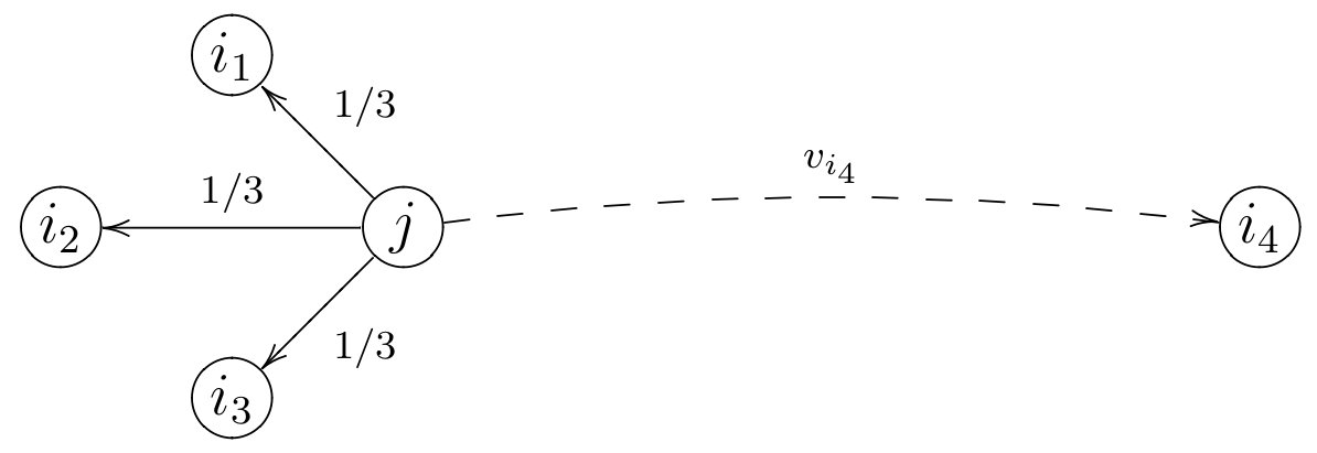
Implement the power and the Krylov (Arnoldi) methods for computing the steady state probability distribution of the “random-surf” random walk on a graph, described by the transition probabilities (see also figure below)

$$ P(X_{n+1} = i | X_{n} = j) = \begin{cases} \alpha \frac{1}{d_j^{\text{out}}} + (1-\alpha) v_i & j\to i\newline (1-\alpha) v_i & j\not\to i, d_j^{\text{out}} > 0 \newline v_i & otherwise \end{cases} $$ where $\sum_i v_i = 1$, $v_i\geq 0$.

When implementing the method pay extra care to ensure that the cost per iteration is at most $O(m)$, where $m$ is the number of edges in the graph. In order to do so, you should write down the transition matrix of the chain $P$ in terms of $A$ (the adjacency matrix) and $v$, the “teleportation” vector.

Assume nodes (states) and edges (links) are given by the London train transportation network, which you can download from the links below:

Edges
Nodes
Description

Observe numerically that:

• The convergence rate of the power method is $O(\alpha^k)$

• The convergence rate of the Arnoldi method is greater than $\alpha^k$

• The convergence of the power method is not affected by the choice of $v$. However, changing $v$ changes the steady state distribution.

• For different values of $v$ select the five “most important” nodes, find out the names of the stations and color them with different colors in the graph drawing.

Code for loading and visualizing the dataset

close all
clear all

%% read the london transport graph
M = dlmread('./dataset/london_transport_edges.txt');

n = max(max(M(:,2)),max(M(:,3)))+1;
A = zeros(n,n);
for row = 1 : size(M,1)
    i = M(row,2) + 1;
    j = M(row,3) + 1;
    w = M(row,4);
    A(i,j) = w;
end


filename = './dataset/london_transport_nodes.txt';
fileID = fopen(filename);
nodes_info = textscan(fileID,'%d %s %f %f');
fclose(fileID);


G = graph(A,'upper');

plot(G,'xdata',nodes_info{4},'ydata',nodes_info{3})